justesen.xyz

The intervention

Your friend is a terrible gambler. He's found two games at the casino and has the spreadsheets to prove he loses money at both. So he starts playing both games, switching between them at random. And starts winning.

This is Parrondo's paradox, described by the Spanish physicist Juan Parrondo in 1996 and formalised by Harmer & Abbott (1999). Two individually losing strategies can combine into a winning one.

The two games

Game A is a simple biased coin. You win $1 with probability p₁ and lose $1 otherwise. Set p₁ = 0.495 — just below fair, so you lose slowly.

Game B is capital-dependent. If your total capital is divisible by 3, you flip a bad coin with win probability p₂ = 0.095. Otherwise, you flip a good coin with win probability p₃ = 0.745.

p₁ = 0.495   ·   p₂ = 0.095   ·   p₃ = 0.745

Game B looks like it should win — you flip the good coin two-thirds of the time. But the Markov chain dynamics push you into the "divisible by 3" state more often than you'd expect, and the bad coin wipes out the gains. Both games lose.

Now play both

Each round, flip a fair coin to decide which game to play — A or B, fifty-fifty. I simulated 1,000 players over 10,000 rounds for each strategy:

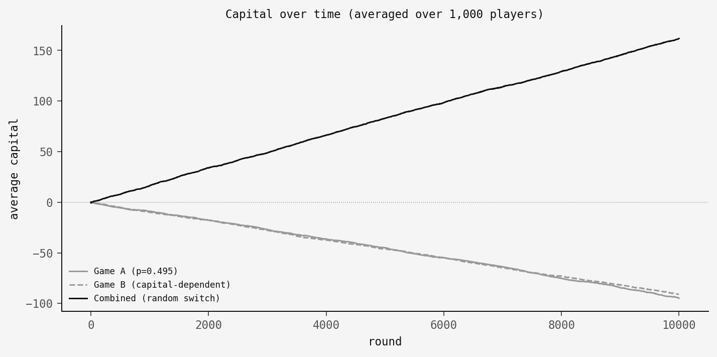
Both games lose on their own. The combined strategy goes up.

Why it works: the ratchet

It comes down to the mod-3 state distribution. When you play Game B alone, the Markov chain settles into a steady state that overweights state 0 — the "divisible by 3" state where you face the bad coin. In my simulation, players spend about 38% of their time in state 0, well above the 33% you'd get from a uniform distribution. That's enough to make the overall expected value negative.

Game A acts as a ratchet. It doesn't depend on capital mod 3, so playing it disrupts Game B's unfavourable equilibrium. It redistributes your capital across the mod-3 states, pushing you away from state 0 and onto the good coin more often:

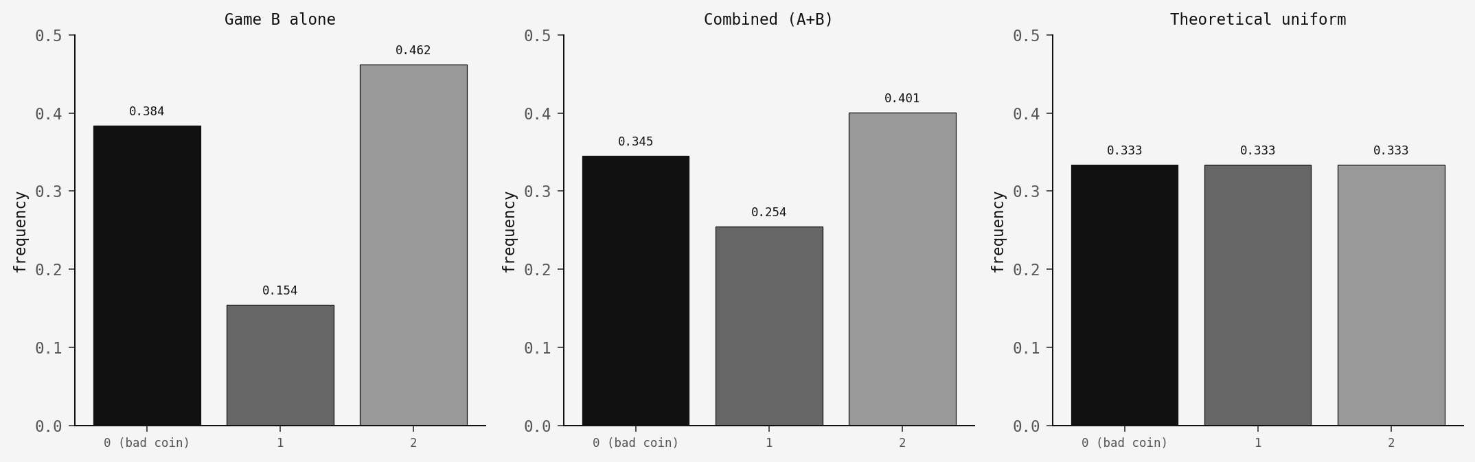
Game B alone: state 0 at 38.4%. Combined: drops to 34.5%, closer to the theoretical 33.3%. That's a small shift, but it's enough to flip the expected value from negative to positive.

How robust is it?

Is this sensitive to the exact parameter values? Here's a sweep across (p₂, p₃) with p₁ fixed at 0.495. The dark region is where the combined strategy wins:

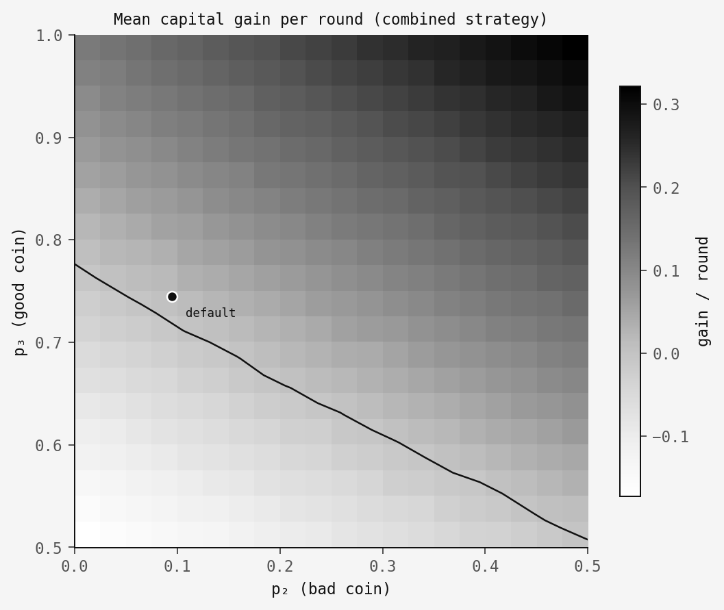
There's a reasonable region above the contour line where the paradox holds. Not a knife-edge.

The code

The core logic fits in a single function:

def play_round(capital, game, rng, p1=0.495, p2=0.095, p3=0.745):
    """Play one round. Returns +1 (win) or -1 (loss)."""
    if game == 'A':
        return 1 if rng.random() < p1 else -1
    else:  # Game B
        if capital % 3 == 0:
            return 1 if rng.random() < p2 else -1
        else:
            return 1 if rng.random() < p3 else -1

Game A checks one probability. Game B checks your capital mod 3 and picks the corresponding coin. The full simulation with all three figures is in code.py.

Takeaway

The point is that combining stochastic processes is not the same as combining their expected values. When the dynamics are state-dependent, mixing strategies can shift the stationary distribution in ways that matter. Here the random switching disrupts an unfavourable equilibrium, and that's enough.

The same kind of thing shows up elsewhere. In biology, fluctuating environments can benefit populations that would decline in either environment alone. In trading, there's Shannon's demon: a portfolio rebalanced daily between cash and a volatile stock can grow even when the stock has zero expected return. The rebalancing, like the game-switching here, profits from the structure of the fluctuations rather than their direction.

Anyway — next time your friend finds two losing games at the casino, maybe check their modular arithmetic before staging an intervention.